If Wishers Were Horses, Beggars Would Ride

The National Cancer Institute (of the NIH) announced this week a large reorganization of its clinical trial system.  As part of the reorganization it announced smaller budgets for running clinical trials.  This reorganization has been coming down the pike for a while now and the smaller budgets are a matter of fact given reduced funding from Washington.

What I found disturbing in the announcement was the repeated claim that new technologies in oncology drugs would reduce the need for large clinical trials.  

According to the announcement

Although the screening tests may need to be performed on very large numbers of patients to find those whose tumors exhibit the appropriate molecular profile, the numbers of patients required for interventional studies are likely to be smaller than what was required in previous trials. That is because the patient selection is based on having the target for the new therapy, leading to larger differences in clinical benefit (such as how long patients live overall or live without tumor progression) between the intervention and control groups.

It is true that breakthrough advances such as the AIDS cocktail or Gleevac can show themselves to be enormously effective even in small trials, but that doesn't mean that we should expect all new drugs or treatments coming into development to be breakthroughs.

It is unclear to me why we should expect that targeted therapies should have larger effects on survival.  I see why we should expect targeted therapies to be more targeted and thus only likely to work for a small subset of patients with very particular genetic mutations in their tumor.  But even if the therapy works on the "bench" it may not have the same effect once it is put into humans.  As the announcement states, targeted therapies will require greater amounts of genetic screening in order to find the right patients.  More over, the total population of patients with a particular genetic mutation may be extremely small.  The future of targeted therapies may well involve smaller clinical trials, but I think NCI is being rather optimistic believing that we won't need large trials.  Today's "Daily News" from ASCO presents a very different view from Don Berry.

Gleevac is the poster boy for new age of targeted therapy, but it is a drug that seems to be exception rather than the rule.  Gleevac was able to solve a very particular genetic problem for a very particular class of cancer patients.  The genetic problems in most common cancers seem to be substantially more complicated and do not seem amendable to single target therapies.  In colon cancer, genetic testing is required for certain drugs, not because these drugs have amazing breakthrough effects, but rather because they don't seem to work when certain genetic mutations are present (see here).

In the mean time non-targeted therapies like immunological therapies are starting to be developed.  Will these therapies also require smaller trial sizes?

Let's hope NCI gets its wishes and all future drugs are breakthrough therapies that don't require large clinical trials and beggars can finally ride.

A New Way to Solve Confounding?

IV Graph from Imbens (2014)

Confounding refers to statistical problem that there is some unobserved characteristic of the patient that is both determining the patient's observed treatment and the patient's outcome.

For example, this study shows that older stage III colon cancer patients are much less likely to receive oxaliplatin as an adjuvant therapy than younger patients.  This may be the reason that in the Medicare data, oxaliplatin is associated with bigger survival effects than in the randomized control trials.  The Medicare data suffers from a confounding problem.  Doctors of sicker patients may be less willing to prescribe oxaliplatin because of its side effect profile.  The observed difference in survival may not be due to the use of oxaliplatin, it may simply be the fact that the non-oxaliplatin patients are sicker.

In the graph to the right, the unobserved variable (patient "sickness") is represented by the red U.  The patient's treatment (oxaliplatin or not) is represented by the black X and the patient's survival is represented by the black Y.  We would like to know whether there is a blue line from X to Y, representing treatment effect of using oxaliplatin on survival.  But we can't determine the treatment effect because U is affecting both X and Y through the red lines from U to X and U to Y.  Sicker patients are less likely to get oxaliplatin (red line from U to X) and sicker patients have lower survival (red line from U to Y).

A standard way to solve the confounding problem is to observe (or introduce) a fourth variable (Z) which is called an "instrumental variable."  As the graph shows, the instrument is some observed characteristic of the patient that determines the patient's treatment choice but is unrelated to the patient's unobserved characteristic or the patient's survival.  In randomized control trials the instrument is the random number generating process that is used to assign patients to treatment arms.

In the Medicare data on the use of oxaliplatin, the instrument may be the date of the diagnosis.  Patient's diagnosed earlier were much less likely to receive oxaliplatin than patient diagnosed at a later date.  By looking at changes in survival over the time period of the introduction of oxaliplatin we can determine the causal effect of oxaliplatin on survival (assuming no other major changes to treatment during the same time period).  

An alternative way to solve the confounding problem is to measure all the confounding characteristics.  If we observe U then we can simply measure the effect of X and U on Y.  If we observe the co-morbidities of the patient we can measure the relationship between the co-morbidities and the use of oxaliplatin on survival.  The problem with this approach is that we may not observe all the confounding factors.

A new paper of mine (see discussion here) suggest an alternative approach.  Instead of attempting to directly measure U, we infer U from observable characteristics of the patient.  Instead of attempting to directly measure the "sickness" of the patient, we look at observable characteristics of the patient like their age and use those signals to determine the distribution of patient's latent sickness type.

This mixture model approach has the advantage of not requiring instruments and not requiring that observe every possible characteristic of the patient that may be determining the treatment choice.

Can Mixture Models Cure Cancer?

Mixture model example from Wikipedia

The other day I was emailing with a friend about my new paper in which I use something called a "mixture model" to analyze the variation in treatment effects.  I'm pretty excited about the idea of using mixture models in this way, but was my friend was somewhat dismissive.

The idea of a mixture model is pretty straight forward.  Imagine observing a distribution where the four distributions pictured to the right were all equally likely and we saw the probability of an outcome less than -2.  For the purple type the probability is 0.5, for the red type it is 0.  For the green type it is about 0.05 and for the blue type it is about 0.1.  So in our data we should see an outcome less than -2 about (0.5 + 0 + 0.04 + 0.1)/4 = 0.16 (about sixteen percent of the time).  

The statistical question of interest is if we observe outcomes less than -2 sixteen percent of the time, can we use this information to decompose the observed probability into the four underlying types that generate the observed data?  Can we tell from our data how many hidden types there are?  Can we tell the proportion of each type?  Can we determine the distribution for each type?

The answer is no.

It is easy to see this.  Imagine that instead of the purple type having a probability of 0.5 that the outcome is less than -2, it is 0.4 and the probability for the blue type is instead 0.2.  The observed probability in the data will again be 0.16.   We can arbitrarily change the underlying type probabilities, as long as the aggregate is 0.64.  All such possibilities are consistent with what we observe.  Similarly, we can change the weights and the probabilities in many different ways and still get the observed sixteen percent we see in the data.

OK, so if we can't decompose our observed data into the underlying distributions, what is the point?

The interesting thing about these models is that with certain information and certain assumptions about how the data is generated, it is possible to decompose the data into the underlying distributions.

Unfortunately, it is very very common to estimate these models when there is not enough data to do the decomposition.  Often the resulting decomposition is coming from arbitrary and non-credible assumptions made by the researcher rather than any actual information in the data.  Worse, it is often unclear how much of what we know about the distribution is due to information in the data and how much is due to the arbitrary assumptions of the researcher.

In 1977, a mathematical statistician, Joseph Kruskal, worked out in this paper, sufficient conditions for the data to provide enough information for the observed distribution to be decomposed into the underlying distributions.  That is, Kruskal presented a set of conditions for when the data and not arbitrary assumptions of the researcher would provide enough information for the decomposition.  More recently, in this paper, signal engineer, Nikos Sidiropoulos, and co-authors presented necessary conditions on the data for the decomposition to possible.

My new paper thinks of their being different types of people, where not only may these different people have different outcomes, but the treatment being tested may have different effects.  When we test a new drug using randomized control trials we generally present the results aggregated over the different types.  If we find that the drug increases survival, we do not know if it increases survival for some people, all people, or most people.  The objective of the statistical analysis is to uncover the different hidden types and ultimately to target particular drugs to particular sub-groups of the population.  The hope is that this can be done without resorting to arbitrary and non-credible assumptions.  My friend remains skeptical.

Can Netflix Cure Cancer?

Neil Hunt of Netflix discusses a number of issues related to the value of randomized control trials to cure cancer.  While Hunt is a bit off on the number of people that take part in clinical trials and about Gleevac, it is a very interesting talk.

Confounded by Confoundedness

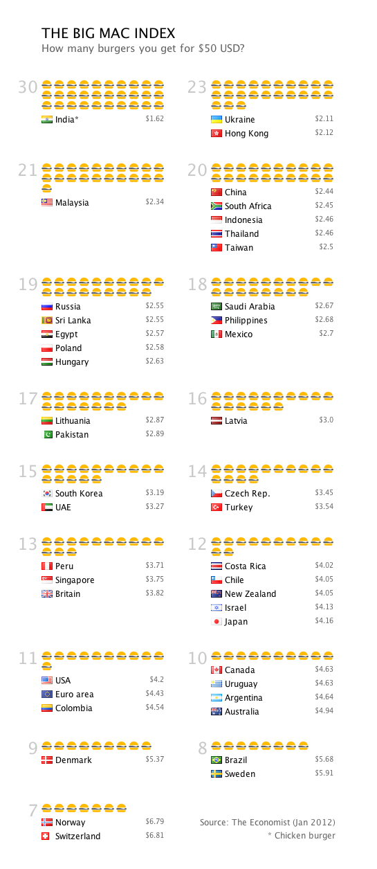
Data based on the Big Mac index by
The Economist -magazine January 2012.

Over the last few weeks I have been confounded by a couple of articles on the health effects of diet.  

One article presented the results of a large diet survey where the health outcomes such as death were matched to the participants who filled out the diet survey.  The article suggested that various healthy diet choices led to major positive health outcomes like not dying.  The article didn't discuss the obvious concerns and skepticism we should have about such a study, on the contrary, the article interviewed various people who said the results bolstered policy recommendations such as food pyramids.

The second article was from a New York Times blogger, George Johnson.  Johnson was attending the American Association of Cancer Research conference and noted that there was little work in which large diet surveys were matched with health outcomes at the conference.  Johnson stated that the lack of interest was due to the problems of interpreting such work.

Observational studies such as large diet surveys with matched health outcomes data suffer from obvious confounding issues.  However, I'm confounded by both the unthinking acceptance of such statistical analysis and the absolute dismissal of such statistical analysis.  Isn't there some middle ground?

For anyone trained in economics the middle ground solution is to find "instruments."  Instruments are not bagpipes, rather they are observable variables for which it is plausible to make the following claim: there is some observational characteristic associated with survey participants that is associated with diet choice but not the health outcome of interest.  For example, some participants may live in France.  

When one lives in France, one tends to have access to French food and French food prices.  For example a French Big Mac is 510 calories, while a US Big Mac is 550 calories.  The US Big Mac is 8% bigger.  The US Big Mac costs $4.20, while the French Big Mac costs $4.43 according to the Big Mac Index.  So if you live in France you get to buy smaller Big Macs for more money than if you live in the US.

The French tend not to be as fat as Americans (see OECD slide here).  One reason is that they face different food choices and different food prices.  Another is that they have different preferences.  Apparently, there exist people in France who do not like Big Macs.

Economists, Aviv Nevo, Rachel Griffith and Pierre Dubois, analyzed differences in food consumption in France and the UK in a forthcoming paper in the American Economic Review.  The authors find that part of the explanation for different food consumption patterns is prices, but part is preferences.  

To the extent diet is determined by the prices faced by the survey participant, then it is likely to be unrelated to the participants preferences and other lifestyle choices like not smoking.  

If we know the geographical location of a survey participant, we can start to unravel whether diet causes cancer or whether diet and cancer are related through other lifestyle choices like smoking.

Inferring Heterogeneous Treatment Effects

People are different.  Different people have different cancers and those cancers require different treatments.  While most oncologists and cancer researchers understand this, it does not stop them from insisting that we must rely on statistical techniques that are not able to measure the effect of these differences on treatment outcomes.

Standard statistical analysis of randomized control trials provides unbiased estimates of the average treatment effect.  Standard statistical analysis of randomized control trials provides no information about the variation in the treatment effect across the patient population.  

To observe variation in treatment effect we would have to observe each patient's outcome with both the treatment that they received and the treatment that they did not receive.  Economists call this the "counter-factual" problem.  The treatment the patient did not receive is counter to the fact.  If in some imaginary world we were able to observe both the factual outcome and the counter-factual outcome then we would look at the difference between them and measure the distribution of the differences.  We would be able to measure the distribution of the treatment effect.  As we live in the real world we do not directly observe the distribution of the treatment effect.

While we cannot directly observe the variation in the treatment effect, we may be able to infer it.

The idea is that the heterogeneity in the treatment effect is being determined by some characteristic of the patient that is unobserved by the statistician.  Further, patients can be categorized into latent or hidden classes according to this unobserved characteristic.  These hidden classes can be inferred from observing certain characteristics of the patients that we know to be associated with the hidden classes.  It has been shown that if we observe a number patient characteristics that are all associated with the hidden classes then we may be able to uncover the hidden classes.  

Analysis based on these ideas have been successfully used in econometrics, psychometrics, biostatistics and computer science.

Here is my foray into the use of a technique called non-negative matrix factorization.  I use the technique to analyze heterogeneous treatment effects in adjuvant therapy for colon cancer.

Adaptive Clinical Trials

Don Berry

At the recent NCCN conference, I was introduced to the idea of an "adaptive clinical trial."  There are a number of ideas that get amalgamated into this general description. One example is that the weighted random assignment into each arm of the trial changes over time in response to trial results.  

For example, the trial may begin by assigning all patients to each of the two arms with probability one half.  However, after say the first year the data suggests patients in one of the two arms have greater survival, at that point the weight increases.  It may be that if probability of surviving 6 months is 5 percentage points higher for the new treatment, then the proportion of new patients assigned to the new treatment arm increases to 60-40.  If at a year, the difference remains, then the percentage may increase to 70-30.  However, if the difference reduces, the percentage of patients assigned to the new treatment arm may fall to 50-50.  On the other hand, if patients in the new treatment arm have one year survival that is 10 percentage points higher, then the percentage of patients assigned to the new treatment may increase to 80-20.

Before talking about the advantages or disadvantages of such a trial design, it is important to remember that current trials accrue patients over time and large trials may take years before they have enough patients.  During this time, information on the value of the new treatment is being carefully accumulated, stored and kept away from prying eyes.  The FDA strongly prefers that data not be available to researchers so as not to lead to biased trial results.  That said, trials often have a data committee who are responsible for looking at the data and deciding whether or not there are severe enough safety problems such that the trial should be stopped.

From a statistical point of view, the trial design has no obvious disadvantages and may have some advantages.  Assignment is still random, and as long as no information on the value of the various treatments leaks to patients or doctors, the trial results should remain unconfounded and unbiased.  One advantage of the trial design is that it may reduce the selection-into-study bias.  Potential patients may be much more willing to sign up for a trial where they know that the probability of being assigned the better arm is increasing in the difference between the trial arms.

Two possible problems are that the power of the trial may be reduced because one of the arms is getting a smaller proportion of the patients.  Another problem is associated with so called "bandit problems."  It is theoretically possible that through statistical coincidence, patients on one of the trial arms start doing very poorly.  This will cause the weights to move away from that arm to the other trial arm.  It may be that the initial poor results would be overwhelmed by later data, had the assignment remained at 50-50 but because of the adaptive design there isn't enough patients being assigned to the trial arm for overwhelming to occur.  While this is not a bias problem, it may mean a greater probability of false-positive trial results.

The FDA raises a number of concerns with such trial designs in this report.   

"Causal Effects" and Randomized Control Trials

One reason for wanting to conduct a randomized control trial is that it provides evidence of the causal effect of a new drug or treatment.  However, if we define "causal effect" as the difference in outcomes a patient would receive on the new drug and the outcome the patient would have received on the alternative, then it is not clear RCTs can provide this information.

Don Rubin points out in this paper that the problem is that we cannot observe the same patient's outcome for both the new drug and for the alternative.  We are limited to observing only the patient's outcome for the treatment that the patient actually received.  

We cannot observe the "causal effect."

Rubin states that all is not lost because it is possible to measure the average treatment effect with an ideal randomized control trial.  The problem, is that the average treatment effect may not provide information on the effect of the treatment on the average patient, the majority of patients or even a plurality of patients.  The average treatment effect averages over the treatment effects of the different patients.

In the comment to this post, Bill provides an example in which 99% of patients live one month shorter on the new drug and 1% of patients live 200 months.  Such a trial will show that on average patients live 1 month longer on the new drug.  This example shows that the average does not have to reflect the outcome for majority of patients or even for a plurality of patients.

In most cancer trials the authors present the difference in median survival between the treatment arms.  I show in this unpublished working paper, that for arbitrary differences in median survival it is easy to find examples in which almost all patients (every patient except 1) their individual outcomes is the opposite of the median difference.

So a positive average treatment effect does not imply even a significant proportion of patient will benefit from the drug and a positive difference in median survival does not imply that a significant proportion of patients will benefit from the drug.

What about other measures, hazard ratios, Kaplan-Meier plots, can any information from the randomized control trial tell us if any reasonable number of patients will benefit from the drug?

Hazard ratios are based on "regression techniques" that make strong parametric assumptions that may not be true in practice.  But even assuming that the parametric assumptions were correct the results only show that some positive number of patients will have some positive benefit from the drug.  Like with the average treatment effect, a proportional hazard ratio is calculated by "averaging" over patients, some of whom may benefit from the drug and some of whom may not.

Kaplan-Meier plots are potentially representations of the marginal probability of survival for each treatment.  If the trial does not suffer from attrition bias or participation bias then the difference in the survival curve at each point in time provides an estimate of the minimum number of people who would benefit from the drug.

If there is attrition bias or selection-into-sample bias then the results from the Kaplan-Meier plots can still be used to provide the minimum number of people who would benefit from the drug.