ATE: What Is It and Why Should You Care?

Arthur Dent is from Earth, which the Encyclopedia
Galactica describes as "mostly harmless."

ATE is economics shorthand for the "average treatment effect" or what Rubin calls the "typical causal effect."  Many think of it as the "casual effect."

ATE is the raison d'etre of randomized control trials.  

I believe that researchers should provide policy makers, doctors and patients with more information than the average treatment effect, but not all economists agree.

In their book "Mostly Harmless Econometrics", Joshua Angrist and Jorn-Steffen Pischke state, 

Even a randomized trial with perfect compliance fails to reveal the distribution of [difference in treatment outcomes]. This does not matter for average treatment effects since the mean of a difference is the difference in means. But all other features of the distribution ... are hidden because we never get to see both [treatment outcomes] for any one person. The good news for applied econometricians is that the difference in marginal distributions, is usually more important than the distribution of treatment effects because comparisons of aggregate economic welfare typically require only the marginal distributions of [treatment outcomes] and not the distribution of their difference.

It is not exactly clear what Angrist and Pischke mean but there is some support their argument.  In his book Public Policy in an Uncertain World, Charles Manski, shows that a policy maker that maximizes a standard social welfare function (trust me it is something economists think policy makers may theoretically do), should only be interested in ATE.

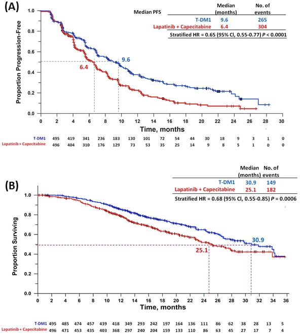
Actual policy makers do not only care about ATE.  Consider the drug Vioxx.   It worked pretty well "on average." It was just the small matter of severely harming a few patients that got it into trouble.

It may be more important to remember your towel than to know the ATE.

Average Probability of Survival Effect

In a previous post, I claimed that it was not possible to estimate the average causal effect on survival for treatments in cancer.  It is not possible because average survival is not observed.  

Moertel et al (1990)

In another post, I pointed that the widely reported median difference in survival has no content.  This is because it is easy to come up with examples in which treatment A has higher median survival than treatment B, and yet almost all patients would live longer on treatment B.

Is there some information that can be garnered from a randomized control trial in cancer that is both measurable and would provide information to regulators, patients and doctors on the likely effect of a treatment?

There is.  It is the "average probability of survival effect".

Consider the figure to the right.  It presents survival probabilities (Kaplan-Meier plots) for the effect of adjuvant chemotherapy for stage III colon cancer patients.  The study was interested in determining whether adjuvant chemotherapy would increase survival for colon cancer patients.  Consider the 4 year mark.  At that point in time approximately 50% of the standard of care arm (observation) had survived, while approximately 70% of patients in the combination with 5-FU arm had survived.

If there is no biased attrition and no biased selection into the study, then we have unbiased estimates of the average probability of surviving to 4 years when given no chemo after surgery (50%) and the average probability of surviving to 4 years when given 5-FU after surgery (70%).  As the difference in averages is equal to the average difference we know that for the average stage III patient, taking a 5-FU based adjuvant chemotherapy increases the 4 year survival probability by twenty percentage points.

Of course, we may not be average and the policy implications of the measure are not clear, but those are discussions for another time.

Is There Any Theoretical Justification for Randomized Contrial Trials in Cancer Research?

No.

There is no theoretical justification for using randomized control trials to test the effectiveness of treatments for cancer in humans.

Donald Rubin

To be clear, the question is not whether it is good to have careful studies or to do replicable analysis.  Those things are good.  The question here is whether randomizing treatment assignment provides any information over and above some other treatment assignment mechanisms.  To be even more clear, the question is not whether randomized control trials are justified in general.  The question is whether they are justified in measuring survival in cancer research.

When justifying the use of randomized control trials statisticians generally point to Harvard's Donald Rubin and his seminal paper "Estimating Causal Effects of Treatments from Randomized and Nonrandomized Studies."  In the paper, Rubin states that "...given the choice between a randomized study and an equivalent nonrandomized study, one should choose the data from the experiment..."

Why?

Rubin says that we should be interested in the causal effect of some treatment.  If we were interested in the causal effect on survival of a new drug, Rubin would define that to be the difference between a patient's survival on the new drug and a patient's survival on the alternative treatment (perhaps the standard of care).  I have no problem with that definition.

But Rubin notes that this difference, the causal effect, cannot be observed.

Houston we have a problem.

So what to do.

This is where the rabbit goes into the hat.  Watch carefully.

Rubin states that instead of the causal effect (which is not observed) we should instead be interested in the "typical" causal effect.  OK.  I'm with you.  Typical sounds reasonable. 

Rubin then states that an "obvious" definition of "typical" is the average difference.  Perhaps.  Rubin then points out that due to the linearity of averages, the average difference is equal to the difference in the average outcome for each treatment.  Further, due to the unconfounded nature of ideal randomized control trials, the average outcome of each treatment arm is an unbiased estimate of the average outcome of each treatment.  

Bob's your uncle.

If we are willing to concede that the average causal effect is the appropriate measure, then that information is provided by an ideal randomized control trial.

Why is cancer different from every other night?

I'm glad you asked, youngest imaginary blog reader.

Cancer is different from every other night because in cancer, people die.  Actually, the statistical problem is caused by them not dying.  Because people don't die we have a censoring problem and we are unable to measure the average survival from each trial arm.  No average, therefore no difference in averages, therefore no average difference, therefore no typical difference, and therefore no dice.

Was EMILIA Biased?

Dr Kimberly Blackwell

In 2012, I got the opportunity to represent Fight Colorectal Cancer as a patient research advocate at the American Society of Clinical Oncologist (ASCO) meetings.  It was an amazing experience.  At those meetings I had the opportunity to see Dr Kimberly Blackwell present findings from the Phase 3 trial measuring the effectiveness of T-DM1 (Kadcyla) for HER2 metastatic breast cancer patients (EMILIA).

Recently, I was looking at data on EMILIA in ClinicalTrials.gov and noticed that the results of trial may suffer from attrition bias.  Just under 1,000 patients participated in the trial with half in the T-DM1 arm and half receiving the combination of Lapatinib and Capecitabine (X+L).  What I noticed was that 48 patients (about 10%) left the X+L arm of their own volition, while only 28 patients (about 6%) left the T-DM1 arm of their own volition.

EMILIA was an "open-label" study, so the patients and their doctors knew what drug they were taking.  If patients who were more likely to do well on T-DM1 relative to X+L, were more likely to stay in the trial, then the results may suffer from attrition bias.  At the 24-month mark there were 111 patients remaining in the T-DM1 arm and 86 patients remaining in the X+L arm.  Some of the difference is due to the difference in survival between the two arms, but some of the difference may be due to difference in patient/doctor choices.  

To the extent it is the second, then we no longer have random assignment between our two comparison groups.  In particular, the patients left in the T-DM1 arm may include a disproportionate number of patients who will live longer on T-DM1 relative to X+L.

Given these observed differences, you may think attrition bias gets a relatively detailed discussion in the New England Journal of Medicine article on the trial or the FDA's approval.  You would be wrong.  The issue is not raised in either forum.

For more discussion of attrition bias in randomized control trials check out this recent paper at BMJ.com or the 2010 National Academies publication.

Can Graphs Cure Cancer?

Judea Pearl

In my previous post, I introduced the idea of a "graph".  Graphs, are a mathematic representation of relationships involving nodes and directed edges.  Graphs are commonly used in a number of branches of science and mathematics.  Economists, like myself, are familiar with graphs from many many many courses of game theory we took in grad school.  However, it was only recently I became aware of the use of graphs in statistics.  I was an immediate convert.

The foremost proponent of the use of graph theory in statistics is the artificial intelligence researcher Judea Pearl.  Pearl argues that graphs provide a simple, clear and coherent representation of many statistical models.

Consider we are interested in the causal relationship between two observable variables (X) and (Y).  We may be interested in the causal effect of a particular chemotherapy (X) on patient survival (Y).  In Figure 1, the causal relationship between X and Y is represented by the directed edge (arrow) from X to Y.  If our data always looked like this, science would be pretty dang easy.  We see some change in chemo treatment and then the resulting change in patient survival and we know how chemo affects survival.

But no.  Science is not that easy.

Unconfounded Graph

Usually, there is some other variable (U) that is some characteristic of the patient that we don't observe.  This may be some genetic factor that we are unable to measure.  This unobserved characteristic also determines survival.  Importantly, this unobserved characteristic may interact with the chemo treatment.  For example, in colon cancer the drug Cetuximab (Erbitux) is only indicated for treatment of KRAS wild-type metastatic patients.  Imagine if we didn't know this genetic marker, we may see some patients do well on Cetuximab and other patients not so well.  

Worse, we may aggregate across patients who are KRAS wild-type and patients who are KRAS mutated and conclude Cetuximab is much less effective than it really is.

Graphs may not directly cure cancer, but I believe they will help statisticians and lay people better understand what the data says about potential cancer treatments.

Instrumental Variables

A graph of an instrumental variable (Z).

If there is one idea that econometricians are rightly proud, it is instrumental variables.  The econometrician, Guido Imbens, has a new NBER working paper, Instrumental Variables: An econometrican's perspective, in which he endeavors to explain instrumental variables to a broader statistical audience.  Note that the paper is technical and not aimed at the lay reader.

Consider the graph to the right.  We are interested in measuring the casual relationship between chemotherapy (X) and survival (Y) (in the graph it is the blue line from X to Y).  That causal relationship may be mediated by some unobserved characteristic of the patient (U) (the red line from U to Y).  It may be that for some patients the drug increases survival while for other patients the drug decreases survival.  The observed relationship between X and Y may also be confounded by U (the red line from U to X).  In observational data we may see some patients (or their doctors) choosing a particular chemotherapy treatment, while other patients who look similar choosing not to have that chemotherapy.  If patient/doctor choice is based on the unobserved characteristic (U) then the observed relationship between X and Y may be biased.

To solve the problem of confounding, economists have suggested using instrumental variables.  There may exist a variable (Z) that determines the treatment but is unrelated to the outcome and is also unrelated to the unobserved characteristics of the patient.  Random assignment in randomized control trials can be thought of as an instrument.  In fact, it may be such a powerful instrument that the red line from U to X actually disappears.  Under random assignment there is no confounding (unconfoundedness).  Imbens discusses various examples of instruments that have been used in economics from weather at sea, to distance from patient to hospital, to lottery number in the Vietnam War draft.  Weather at sea may affect the price of fish by affecting the supply of fish in the market but not the demand for fish.  Distance from patients to the hospital may affect the patients willingness to get a particular treatment but not the outcome of the treatment.  Lottery number in the draft may affect a potentially draftees willingness to go to college but not their wages post college (conditional on going to college).

Most instrumental variables do not completely remove the line from U to X.  They do not completely remove the confounding in the data.  Nevertheless, economists have shown that these variables can improve inference with confounded data.  Thus, instrumental variables may allow the researcher to make inference from observational data or RCTs affected by selection-into-study bias (participation bias) or attrition bias or non-compliance bias. 

Can Observational Data Measure Drug Effectiveness?

Survival and drug use among AIDS patients on
California Medicaid.

It is not often that a graph presented in an economics paper makes me tear up.  But the one to the right always does. Economists, Mark Duggan and William Evans, present this graph in their paper on the effectiveness of drug treatments for AIDS.  The graph shows the change in quarterly mortality for California AIDS patients before and after the introduction of the AIDS cocktail (HAART) in 1996.  The graph shows that quarterly mortality drops from 8% to 2% in the four years around the introduction of HAART.  The graph is based on claims data in California's Medicaid program.

Often in science we are interested in measuring the causal effect of some proposed treatment or policy.  For example, we may be interested in whether HAART causes AIDS patients to live longer.  That is, if we give a particular patient HAART would that patient live longer than they would have lived if they had not received the treatment.  In his book, Causality, Judea Pearl argues that to test whether or not a casual relationship exists we need to conduct an "experiment" where the researcher has the ability to adjust one variable and observe what happens to the variable of interest.  If we want to test the causal relationship between HAART and survival, Pearl says we should conduct an experiment where the researcher is able to control whether or not a patient receives HAART.

Some economists argue that the experiment does not have to be a randomized control trial, rather it could be a natural experiment.  A natural experiment is like a randomized control in that some sub-group of the population of interest receives one treatment, while a different sub-group receives a different treatment.  Importantly, all people in each sub-group have no choice about which treatment they receive.  Moreover, the two sub-groups are otherwise similar (except for the treatment they receive).  The difference is that the experiment occurs naturally in the world.  That is, there is something that happens in the world or some characteristic of the world that leads to different treatment for different sub-groups.

In Duggan and Evans (2008), that characteristic is time.  Prior to January 1996, HAART did not really exist.  It wasn't a treatment option unless the AIDS patient happened to be on AZT and in a clinical trial for Epivir or a protease inhibitor.  After the FDA allowed Epivir and various protease inhibitors on to the market, HAART became generally available.  The graph shows as the use of HAART increased from 0% to over 50% population of California AIDS patients, quarterly survival for these patients fell from 7% to 2%.

While this is compelling evidence that HAART had some causal effect on the survival of AIDS patients it may be harder to determine the extent of that effect or how that effect may vary across patients.  One thing that is clear in the graph is that there is some decrease in quarterly mortality prior to HAART becoming generally available.  That decrease may have been due to the availability of HAART to the clinical trial population which for AIDS peaked at 30% of the population (see previous post).

It is interesting to note that results from one of the first randomized control trials on the effect of combination therapy was published in September 1997.  By the time of publication, HAART use had already hit 50% and quarterly mortality had already fallen to 2%.

Selection-Into-Study (SIS) Bias

Two friends of mine are currently looking for a clinical trial to participate in.  Unfortunately, they are undertaking this search because the current standard of care in metastatic colon cancer is not working for them.  Ironically, if and when they find a randomized control trial, one of the treatment arms is likely to be the current standard of care.

Who exactly participates in randomized control trials for cancer?  Why do patients choose to find a randomized control trial?  Which trial do they choose?

Patient participation rates by drug type for AIDS before and after
HAART.

In an unpublished working paper, Anup Malani and Tomas Philipson, present compelling evidence that the introduction of the AIDS drug cocktail (HAART) in 1996 dramatically affected the willingness of AIDS patients to participate in clinical trials.  In the lead up to the release of HAART on to the market, participation in clinical trials rose to an amazing 30%, however in the next ten years after the introduction of HAART, participation fell back to 5%, about half of what it had been in 1990.

If patients are spending time and energy selecting to participate in a particular study, then that study may suffer from selection-into-study bias.  Following in the tradition of the great Art Goldberger, I believe that if readers are to take an issue seriously, then that issue needs to have an exotic polysyllable name.  While, it is no where near as clever or as funny as Goldberger's micronumerosity, it is hoped that with the help of the double-hyphenated (acronym enhanced), selection-into-study (SIS) bias, we may make progress on a serious issue in randomized cancer trials.

To highlight the concern with SIS bias consider one of the most famous uses of randomized control trials in economics, the Lalonde study.  The study recruited people into a training program and then randomized those recruited into the study into two trial arms.  One group received training and the other group did not.  The researchers collected wages for each of the participants in the study both before and after the training program.  Lalonde then compared the results from the two trial arms to a sample of similar people who did not participate in the program but who did participate in a large nationally representative survey of wages over the same period.

If the group of people who decided to participate in the study differed substantially from general population then the results of the Lalonde study would be biased, making the results difficult to interpret.  That said, the study does provide a possible test for SIS bias.  If those who participated in the study believed that their incomes were likely to be higher with training than without, then we should see that in the data.  In fact, those that received training had a greater probability of a larger income increase than those who were randomized into the arm that did not receive training.  Of course, this result is perfectly consistent with the fact that training increases income.  But what if training only increases income for those who believed it would?  Unfortunately, there is no easy way to determine whether we are observing an average effect for the population or a selection-into-study effect.

There may be another way to test for SIS bias.  A researcher could use distance travelled by study participants.  The researcher can split study population between those who travelled a long distance and those who did not, and test whether the "treatment effect" is larger for those who travelled farther.  If it is, then the study may suffer from SIS bias.  We can think of distance as a "cost" of participating in the trial.  Patients who travel further, give up more in order to participate and may believe that they will have better outcomes than the standard of care.  Note that this test is only valid if it reasonable to assume that treatment outcomes are not associated with patient distance from the trial center.

Can We Learn Anything from Cancer Trials?

Results from EMILIA Trial for T-DM1.

My previous post suggests that it is not possible to learn anything about the survival benefit of new treatments for cancer from randomized clinic trials.  This is not true.

It is possible to learn some limited information about relative survival benefits from randomized control trials.

It is possible to "bound" the proportion of patients who would live longer on the new treatment from the data.  We can use a mathematical relationship known as the "Frechet-Hoeffding bounds''. 

These bounds imply that minimum proportion of the population sampled by the randomized control trial who would benefit from the new treatment is equal to the maximum difference in the survival curves at each point in time.

For example, in the figure we see that at the 12-month mark, the survival difference is 6.8 percentage points, while at the 24-month mark the difference is 12.9 percentage points.  From this we know that at least 12.9% of the population sampled would live longer on T-DM1 versus capecitabine and lapatinib.

From the EMILIA trail we learn that between 12.9% and 100% of the population of metastatic breast cancer patients sampled would live longer on T-DM1 versus the alternative.  Another way to say this, is that we know between 0% and 77.1% of patients would live longer on capecitabine and lapatinib than on T-DM1.

Note that bounds may be even wider than suggested above.  Firstly, our estimate of the bounds may be wider due to sampling variation (which I have not calculated).  Second, the Frechet-Hoeffding bounds result is reliant on the fact that there is no biases in the trial data.   Information reported on ClinicalTrials.gov suggests that 72 patients left the trial of their own decision, 28 from the T-DM1 arm and 48 from the X+L arm.  This unbalanced attrition may cause the results at the 2-year mark to be biased.  I discuss the effect of this bias in this unpublished working paper.

Median Survival Benefit: Meaningless or Mostly Meaningless?

Results from the EMILIA trial on the use of T-DM1

.

You don't have to look hard in cancer research to see claims that some new treatment or other, increases median survival (for example see here).  Generally, authors or journalists claim that the new treatment causes an increase in survival because data from a randomized control trial shows that median survival for patients who received the new treatment is higher than median survival for patients who received the alternative treatment (often the current standard of care).

This is unfortunate because differences in median survival do not indicate anything.

I show, in this unpublished working paper, that it is a simple matter to come up with a mathematical example in which treatment A has greater median survival than treatment B, yet (almost) everyone in the data would live longer if they received treatment B.

Granted, this is just an example.  However, this one example shows that observing differences in median survival does not prove that most, some or even (almost) any patients would live longer on the treatment with the higher median survival.

Why the heck are median survival differences presented in cancer research?

My best guess is that people got a little confused.  It is well known that for idealized randomized control trials, the difference in average survival between treatment groups is equal to the average survival difference.

Difference in averages = Average of differences

Economists call the average of the difference, the "average treatment effect."  It gives a sense of how the "average" patient in the population would respond to a change in the treatment regime she is given.

The problem comes about because the average is unavailable - everyone in the trial must die for the average to be known (without making strong parametric assumptions).  As this would take a long time, even in cancer trials, we are left with measuring things about the distribution that are not averages.  Maybe the thought process went something like this, "medians are like averages, perhaps the difference in median survival between treatment groups is equal to the median survival difference?"

It isn't.

What is the alternative?  I don't know the answer, but we should stop presenting differences in median survival as representative of something.